Transitland is an open data platform that aggregates data from transit providers around the world. Transitland provides an API that can be used to perform queries such as:
- find all the bus stops within a bounding box (geographic region)
- find all the subway routes operated by a particular transit agency
- find all the scheduled trips between two given stops
The Transitland API is powerful. Users can combine multiple API queries to create complex analyses and web maps. In this tutorial, we'll query the Transitland API and combine multiple results into a single XYZ space in order to create an interactive web map of subway routes and stations with frequent service.
This tutorial assumes an advanced level of skill.
What you'll learn
- How to query the Transitland API.
- How to upload Transitland API query results to an XYZ space.
- How to combine multiple Transitland API query results in an XYZ space.
- How to create a web map with interactive filtering from an XYZ space.
Prerequisites
- HERE XYZ account
- Basic familiarity with a terminal/command-line interface
- Basic familiarity with web service APIs
The Transitland API provides access to a wide variety of information about public transit resources, and each API endpoint provides a number of query parameters for filtering the results or including additional details. In this tutorial, we'll use the Stops and Routes endpoints to build an interactive map that visualizes the frequency of service on each route and the wheelchair accessibility for each stop. Transitland even includes stops for gondola and ferry routes!
Stops API Endpoint
The Stops endpoint is at https://transit.land/api/v1/stops Try opening this URL and you should see the following JSON-formatted response:
{
      "stops": [
        {
            "created_at": "2016-02-06T20:08:39.818Z",
            "created_or_updated_in_changeset_id": 12294,
            "geometry": {
                "coordinates": [
                    -121.945154,
                    38.018914
                ],
                "type": "Point"
            },
            "geometry_centroid": {
                "coordinates": [
                    -121.945154,
                    38.018914
                ],
                "type": "Point"
            },
            "geometry_reversegeo": null,
            "name": "Pittsburg/Bay Point",
            "onestop_id": "s-9qc2314hpz-pittsburg~baypoint",
            "operators_serving_stop": [
                {
                    "operator_name": "Bay Area Rapid Transit",
                    "operator_onestop_id": "o-9q9-bart"
                }
            ],
            "osm_way_id": 47228512,
            "parent_stop_onestop_id": null,
            "routes_serving_stop": [
                {
                    "operator_name": "Bay Area Rapid Transit",
                    "operator_onestop_id": "o-9q9-bart",
                    "route_name": "Antioch - SFIA/Millbrae",
                    "route_onestop_id": "r-9q9-pittsburg~baypoint~sfia~millbrae"
                }
            ],
            "served_by_vehicle_types": [
                "metro"
            ],
            "tags": {
                "osm_way_id": "47228512",
                "stop_url": "http://www.bart.gov/stations/PITT/",
                "wheelchair_boarding": "1",
                "zone_id": "PITT"
            },
            "timezone": "America/Los_Angeles",
            "updated_at": "2018-09-20T14:21:06.944Z",
            "wheelchair_boarding": true
        }
    ]
}
This is the record for one stop location. The stop name is Pittsburg/Bay Point, and the stop is served by the Bay Area Rapid Transit operator and by the Antioch - SFIA/Millbrae route. The API response also includes information about the geographic location, timezone, accessibility, and other details.
Routes API Endpoint
Likewise, the Routes endpoint is at https://transit.land/api/v1/routes. The response (omitted here for brevity) is similar to the Stops API, and provides information about the route's shape, transit operator, visited stops, and accessibility information.
Switching to GeoJSON Format Response
HERE XYZ expects data in GeoJSON format, so let's switch the API response format from JSON (the default) to GeoJSON. Use the following URL: https://transit.land/api/v1/stops.geojson. Try opening this in your web browser. You should see the data for 50 stop locations, with each stop as a Feature inside a GeoJSON FeatureCollection. The Routes API endpoint can also respond with GeoJSON, using the same technique: https://transit.land/api/v1/routes.geojson
Filtering API Results Using Query Parameters
By default, most Transitland API endpoints return the first 50 matching results for a query. The database is actually quite large — in fact, you can query using total=true and see that there are over 1.7 million stops. What if you want to query for stops in a particular place? You can supply one or many query parameters to do so.
Filtering by bounding box
Most Transitland APIs allow basic geographic filtering by providing a simple bounding box with the bbox query parameter. A bounding box is a rectangle defined by its two most distant corners. For example, to query for stops in the Chicago Area:
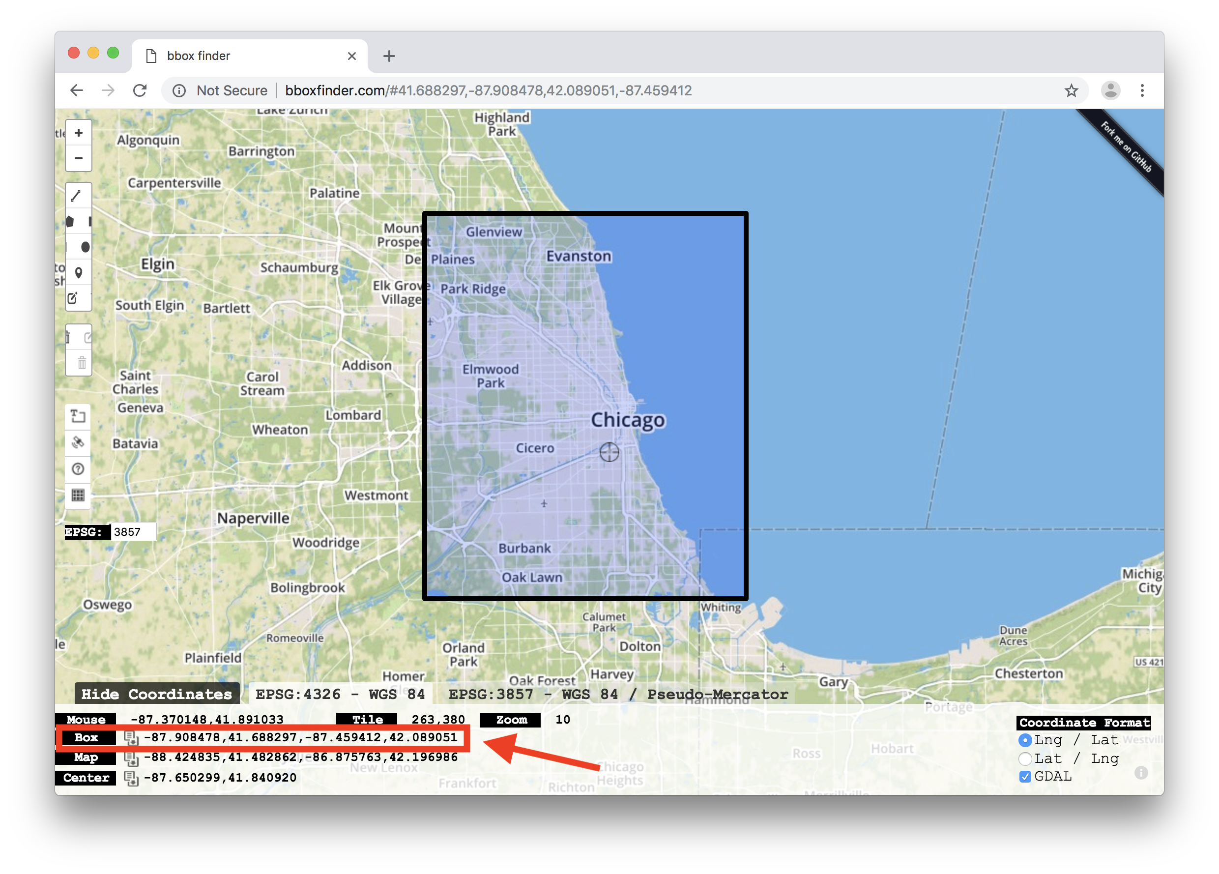
The above bounding box is represented as -87.908478,41.688297,-87.459412,42.089051 (highlighted in red on the screenshot.) This defines the outer corners of the bounding box in the format min longitude, min latitude, max longitude, max latitude.
Next, to query for stop locations within this bounding box, use this value for the bbox query parameter: https://transit.land/api/v1/stops.geojson?total=true&bbox=-87.908478,41.688297,-87.459412,42.089051
There are a total of 18,714 stops in this bounding box.
Filtering by transit mode
Transitland also allows filtering by transit vehicle type, such as subway, bus, light rail, etc. In the Stops API, this filtering is done by specifying the served_by_vehicle_types query parameter. The Transitland documentation provides a list of known transit modes.
The served_by_vehicle_types parameter can be added in addition to the bbox parameter; for example, to select only metro stops (mass rapid transit, including subways and elevated trains) in our bounding box: https://transit.land/api/v1/stops.geojson?bbox=-87.908478,41.688297,-87.459412,42.089051&served_by_vehicle_types=metro.
The Routes API provides the vehicle_type parameter which accepts the same values: https://transit.land/api/v1/routes.geojson?bbox=-87.908478,41.688297,-87.459412,42.089051&vehicle_type=metro.
Now that you're able to retrieve GeoJSON results from the Transitland API, there are multiple ways to upload this to your XYZ space for visualization and analysis. The most powerful way of doing so is through the HERE CLI.
Using the HERE CLI, run the following command to create a new space:
here xyz create -t 'Transitland Map'
This will return an ID for a new XYZ space, which in this example is e9PEZgZg:
xyzspace 'e9PEZgZg' created successfully
We will be using this XYZ space ID in subsequent steps, so assign it to the environment variable $SPACE_ID.
export SPACE_ID=<returned space id>
The here xyz upload command takes GeoJSON input and adds the features to the given XYZ space ID. The input can be either a local file or a remote URL. By entering a URL, you can use the HERE CLI to query the Transitland API. This example queries the Transitland Stops API and adds the features from the response to your XYZ space:
here xyz upload $SPACE_ID -f "https://transit.land/api/v1/stops.geojson?bbox=-87.908478,41.688297,-87.459412,42.089051&served_by_vehicle_types=metro"
Try changing the bbox coordinates to your own bounding box.
View a Basic Map using GeoJSON Viewer
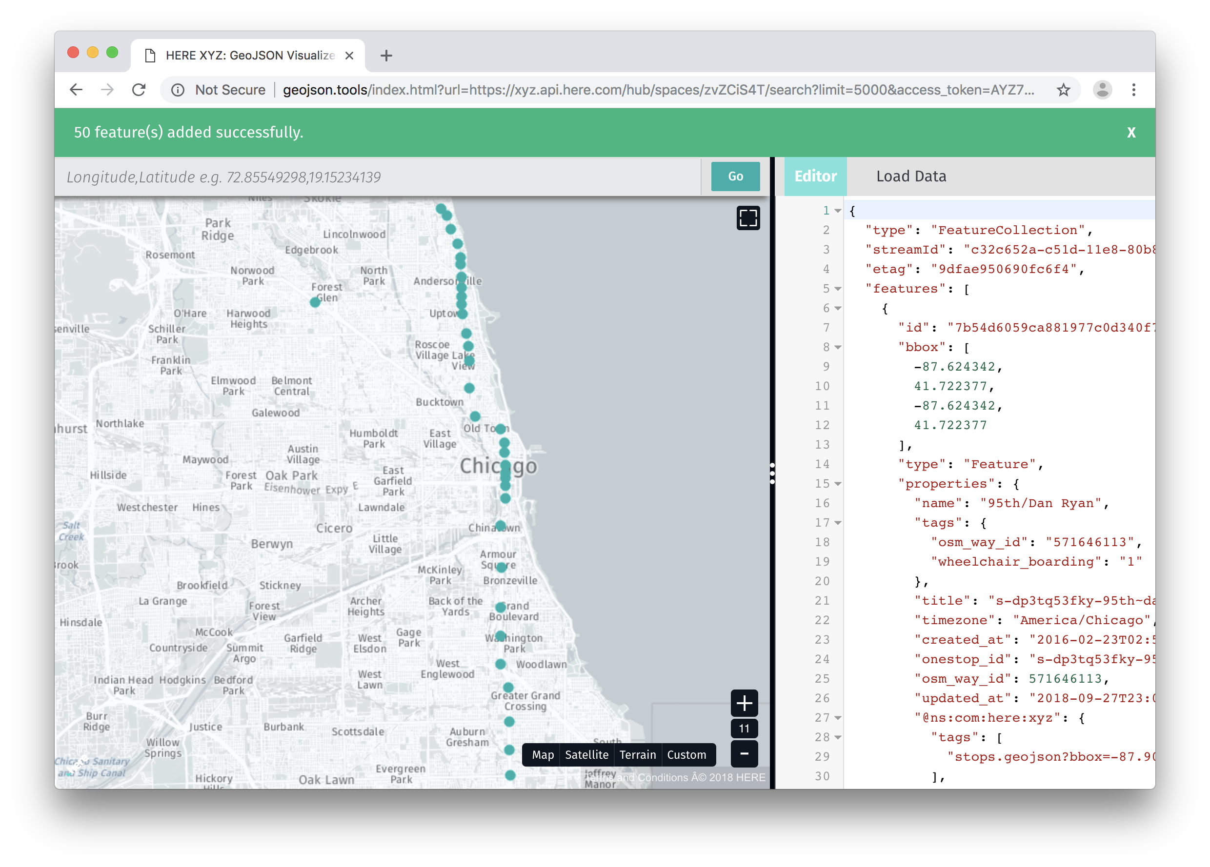
To view the contents of your XYZ space at any time, run the following command to open the GeoJSON Viewer:
here xyz show $SPACE_ID -w
Now we can see stop locations within our bounding box:
The combination of the Transitland API and the HERE CLI is powerful. You can run multiple here xyz upload commands and all of the results will be combined within the same XYZ space.
When you combine multiple Transitland queries into the same output, the same stop or route may be present in more than one query result. For example, queries for two different but overlapping bounding boxes. However, each Transitland entity has a globally unique identifier called a Onestop ID. In the GeoJSON response format, the Onestop ID is available as the feature id. When the -o option is specified for uploading, XYZ uses this ID, matches data across uploads, and updates any existing records.
This example queries the Routes API using the same bounding box as before, and adds the results to our XYZ space:
here xyz upload $SPACE_ID -o -f "https://transit.land/api/v1/routes.geojson?bbox=-87.908478,41.688297,-87.459412,42.089051&vehicle_type=metro"
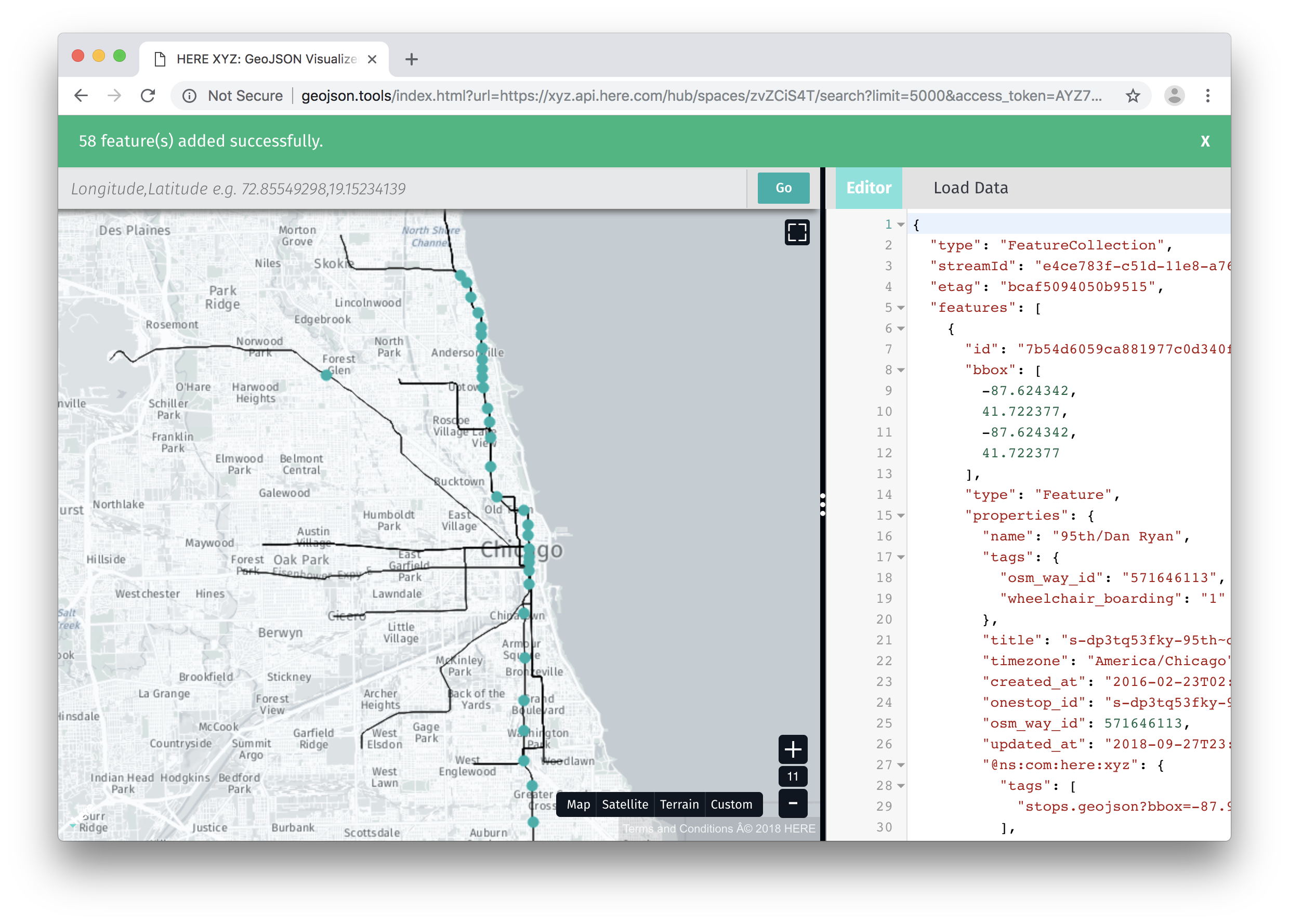
Try running additional Transitland Stops API queries, uploading them to your XYZ space, and viewing the results in the GeoJSON Viewer.
Just because you know where a bus stop is located doesn't mean you necessarily know when you'll be able to ride a bus. To understand a transit network, you need both geographic and temporal information. The Transitland Schedule API is quite sophisticated and allows many types of complex queries. For example, you can query for all the possible times a bus route travels between two given stops. The Routes and Stops APIs also provide access to schedule data, and can include summarized schedule information in the response. For this tutorial, we will use the Routes API headway query parameters to include statistics about the level of service for each route.
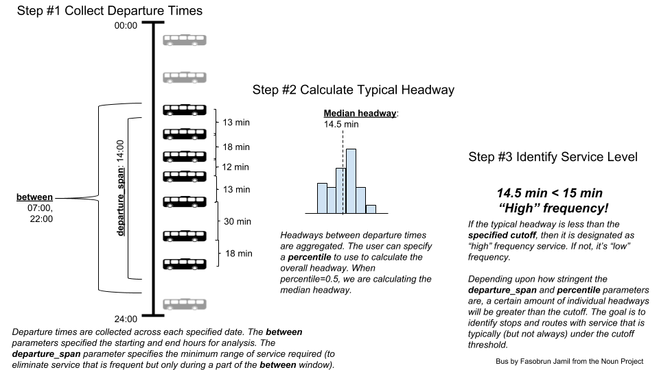
"Headway" is the amount of time between two trips to the same transit stop. In other words, it's how long you'll likely have to wait at a stop for the next bus or train, if you just missed the previous one. Here's a digram of how Transitland computes the typical headway between two stops:
To attach headway information to routes, you need to add two query parameters to your API query:
include=headwaysspecifies that you want to include headway information (it's not included by default, since it takes extra time to compute)headway_dates=2018-09-18specifies the date (or dates) for which you want to compute headways (you can include multiple dates separated by commas)
Here's the command you'd run to fetch routes within a bounding box, including typical headways for September 18, 2018:
here xyz upload $SPACE_ID -o -f "https://transit.land/api/v1/routes.geojson?bbox=-87.908478,41.688297,-87.459412,42.089051&vehicle_type=metro&per_page=10&include=headways&headway_dates=2018-09-18"
Remember, even if you have uploaded these routes, XYZ will merge together duplicate records using their Onestop IDs when the -o option is specified.
Now open these results in the GeoJSON Viewer:
here xyz show $SPACE_ID -w
Click on a route to view its properties. In the following screenshot, we've clicked on the Blue Line route. Then in the object properties panel (upper left), we expanded headways to list out the headway times associated with this route on the given date in September 2018:
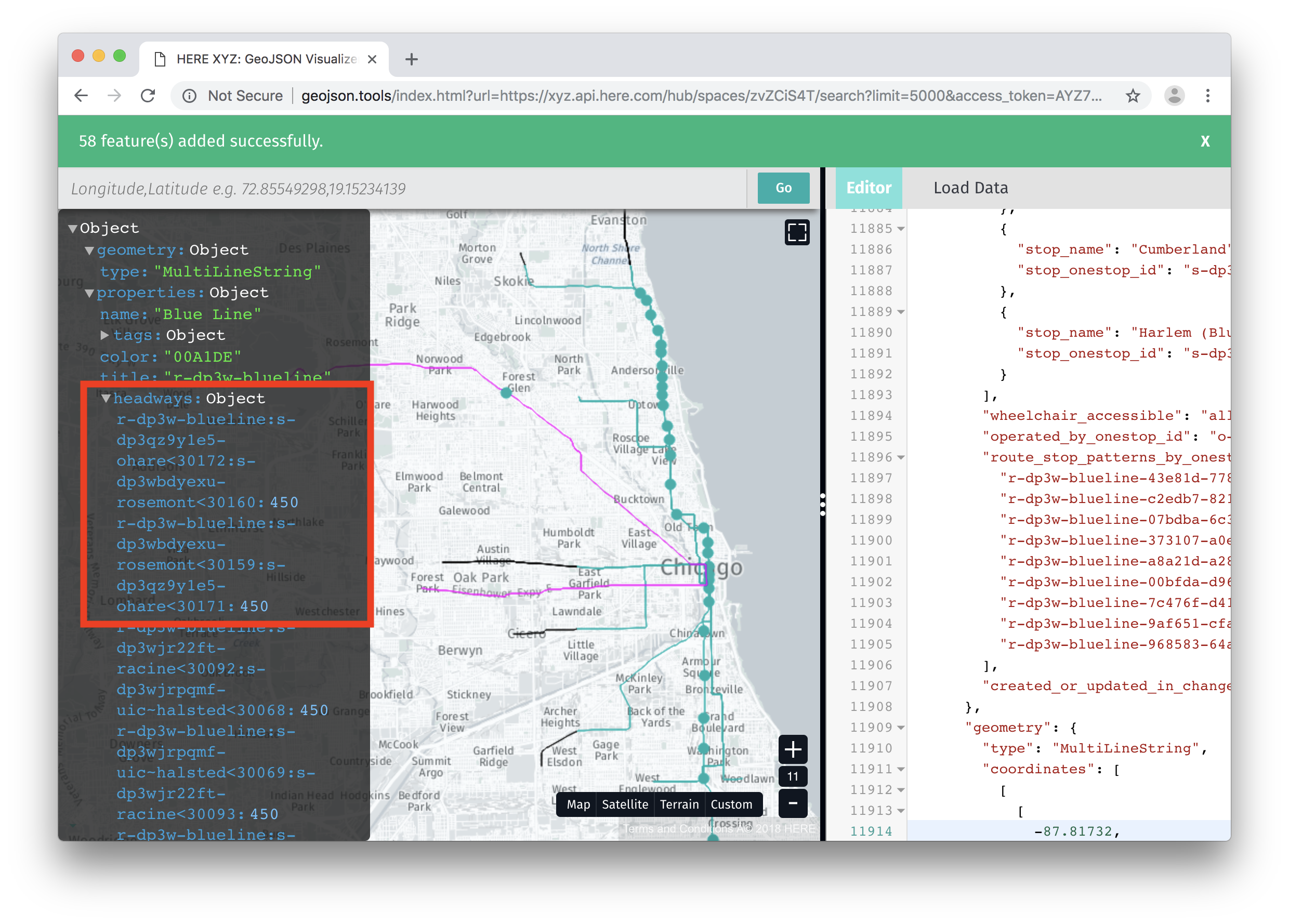
The headway property contains typical headways between all stop pairs on this route, formatted as <route>:<stop1>:<stop2> = headway.
For example, r-dp3w-blueline:s-dp3wbdyexu-rosemont<30159:s-dp3qz9y1e5-ohare<30171 = 450 shows that on the Blue Line route (r-dp3w-blueline), the median time between trains from Rosemont Station (s-dp3wbdyexu-rosemont<30159) to O'Hare Station (s-dp3qz9y1e5-ohare<30171) is 450 seconds on September 18th, 2018. In other words, if you stand on the Rosemont platform all day with a stop watch and counter in hand (tremendously exciting), typically there will be a Blue Line train heading in the direction of O'Hare every seven and a half minutes.
The headways property is somewhat complex — too complex to be filtered using XYZ tags. However, it is possible to use the XYZ API together with some custom JavaScript to to filter stops by headway values.
Let's expand the previous queries by building a global map of all subway routes and stops. Remove the bounding box and run our stops query again: https://transit.land/api/v1/stops.geojson?total=true&served_by_vehicle_types=metro
We can see that there are currently 7,027 subway stops in the Transitland database, a bit too large to fit into a single request. These results can be paginated through using the offset query parameter, for example, offset=50 to load the second page of results. However, as a convenience, the Transitland API includes a URL for the next page of query results. This URL is available in the .meta.next value; for this example: https://transit.land/api/v1/stops?offset=50&per_page=50&served_by_vehicle_types=metro&sort_key=id&sort_order=asc
We will use the .meta.next URL to write a simple shell script to page through all the results and upload to our XYZ space:
url="https://transit.land/api/v1/stops.geojson?served_by_vehicle_types=metro"
while [ "$url" ]; do
    resp=$(curl -s ${url})
    url=$(echo $resp | jq -r '.meta.next // empty')
    echo $resp | here xyz upload -o $SPACE_ID
done
This shell script sets an initial URL, uses curl to make the API request, and then parses the JSON response to get the .meta.next URL for the subsequent page. The response data is then passed to here xyz upload through stdin and uploaded to our XYZ space. This request and upload process loops as long as the response contains a .meta.next URL to the next page. Check that you have both the curl and jq commands available, then save this script as fetch-stops.sh and run it using:
/bin/bash fetch-stops.sh
You should see output from here xyz upload after each iteration.
We will use a similar process to load all subway routes. The Routes API uses the vehicle_type query parameter to filter by travel mode. However, let's also request headway information for each subway route to visualize later. As mentioned previously, headway calculations can take some time on the server, so we will lower our results per page to 5 using per_page=5 to avoid Transitland API timeouts:
url="https://transit.land/api/v1/routes.geojson?vehicle_type=metro&include=headways&headway_dates=2018-09-18&per_page=5"
while [ "$url" ]; do
    resp=$(curl -s ${url})
    url=$(echo $resp | jq -r '.meta.next // empty')
    echo $resp | here xyz upload -o $SPACE_ID
done
Save this script as fetch-routes.sh and run as before. This may take slightly longer to complete; you should end up with about 318 subway routes in the end.
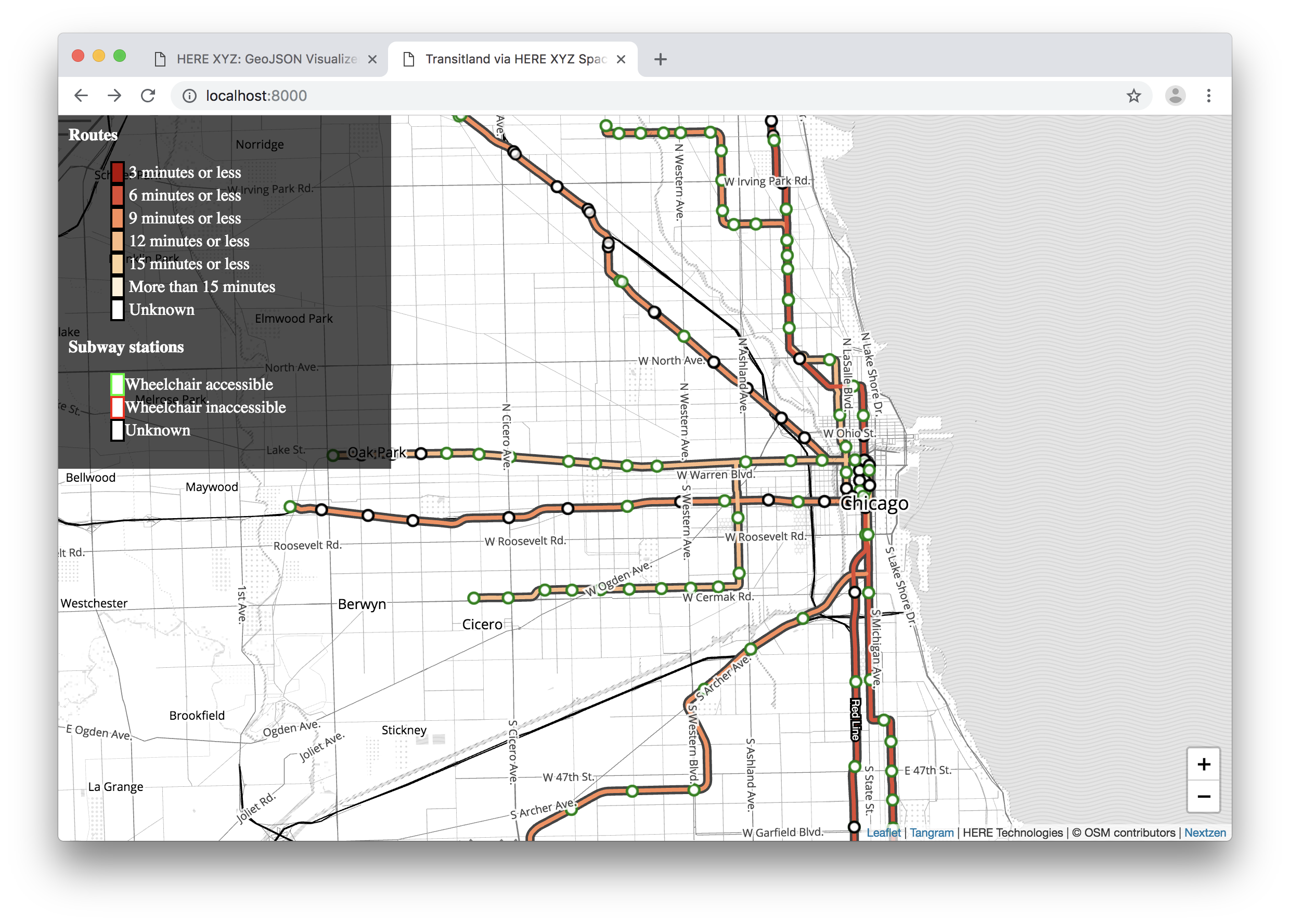
Now that we have populated our XYZ space with transit data, we will visualize this data using a simple web map. Routes will be drawn using a color map that represents typical headways and level of service for each line, and stops will be drawn as green or red to show if wheelchair access to the platform is possible.
For this tutorial, we will use Tangram as the map renderer. Tangram is a flexible WebGL-based mapping engine which can accept input in a variety of formats, including HERE XYZ spaces. Tangram provides sophisticated map rendering through the use of a "scene file", a description of the map sources, styles, and behaviors in YAML format. Please check out the complete Tangram documentation for a additional details and demos.
Our map will consist of three files: index.html, index.js, and scene.yaml for the Tangram scene file. The subsequent sections will walk you through the contents of each file, explaining key details. Comments in each file will explain the intended style or behavior. Save all of these files in the same directory.
Starting a local web server
Please note that due to browser security models, Tangram scene files must be loaded over the network. The easiest way to satisfy this requirement is to start a local web server in the same directory as your files, for example by running Python's SimpleHTTPServer:
python -m SimpleHTTPServer
This will start a web server, which you can access as http://localhost:8000. If you run this command in the same directory as index.html, your web map will load automatically.
index.html
This index.html file provides just enough scaffolding to draw our map. It loads Leaflet (Tangram is instantiated as a Leaflet plugin), Tangram itself, and then our index.js JavaScript which will initialize the map. The document also provides a simple legend for the style we will use for routes and stops.
<!doctype html>
<html>
<head>
<title>Transitland via HERE XYZ Spaces</title>
<script src="https://unpkg.com/leaflet@1.3.3/dist/leaflet.js"></script>
<script src="https://unpkg.com/tangram/dist/tangram.min.js"></script>
<link rel="stylesheet" href="https://unpkg.com/leaflet@1.3.3/dist/leaflet.css" />
<style type="text/css">
body {
margin: 0px;
padding: 0px;
}
#map {
width: 100%;
height: 100vh;
}
.legend {
position: absolute;
top: 0px;
left: 0px;
width: 300px;
padding: 10px;
color: white;
background: rgba(0.9, 0.9, 0.9, 0.7);
z-index: 1000;
}
.legend ul {
list-style: none
}
.legend span {
display: inline-block;
background: white;
border: solid 2px black;
width: 10px;
}
</style>
</head>
<body>
<div id="map"></div>
<div class="legend">
<div>
<strong>Routes</strong>
<ul>
<li><span style="background:#b30000"> </span> 3 minutes or less</li>
<li><span style="background:#e34a33"> </span> 6 minutes or less</li>
<li><span style="background:#fc8d59"> </span> 9 minutes or less</li>
<li><span style="background:#fdbb84"> </span> 12 minutes or less</li>
<li><span style="background:#fdd49e"> </span> 15 minutes or less</li>
<li><span style="background:#fef0d9"> </span> More than 15 minutes</li>
<li><span style="background:#ffffff"> </span> Unknown</li>
</ul>
<strong>Subway stations</strong>
<ul>
<li><span style="border-color:#00ff00"> </span>Wheelchair accessible</li>
<li><span style="border-color:#ff0000"> </span>Wheelchair inaccessible</li>
<li><span style="border-color:#000000"> </span>Unknown</li>
</ul>
</div>
</div>
<script src="index.js"></script>
</body>
</html>
index.js
The JavaScript for this tutorial is just enough to create a Leaflet and Tangram map, which then draws the map based on the scene.yaml file. The initial map view will be of the Chicago area.
// Initialize Leaflet and Tangram, using scene.yaml as the style
var map = L.map('map', {zoomControl: false});
var layer = Tangram.leafletLayer({
scene: 'scene.yaml',
attribution: '<a href="https://mapzen.com/tangram" target="_blank">Tangram</a> | HERE Technologies | © OSM contributors | <a href="https://nextzen.org/" target="_blank">Nextzen</a>',
});
layer.addTo(map);
// Place the zoom controls on the bottom right corner.
L.control.zoom({
position:'bottomright'
}).addTo(map);
// Initialize the view to Chicago, level 12
map.setView([41.87, -87.66], 12);
scene.yaml
The key file in this example is the scene file, scene.yaml. Please see the Tangram documentation for a full reference.
The scene file defines a vector tile base map, and draws this layer using the Refill style developed at Mapzen. Our XYZ space is defined as the second data source. Make sure to replace <SPACE_ID> with your own SPACE_ID, and replace <ACCESS_TOKEN> with your own access token.
Our XYZ space will be drawn on top of our base map, as two layers: routes and stops. The filter defines which features will be drawn in each layer, and draw specifies the style. Both of these layers will use Tangram's ability to load in-line JavaScript to dynamically determine the drawing style for each feature. The routes color function takes a color map, defined as an array of hex colors from Colorbrewer, and a headway time (in seconds) to use for each color. The stops layer likewise contains a JavaScript function to draw each stop feature with a red, green, or black outline based on the value in the wheelchair_boarding property. The stops layer will only be shown at zoom level 12 and above, to avoid cluttering the map when zoomed out.
import:
  # Mapzen Refill style
  - https://www.nextzen.org/carto/refill-style/refill-style.zip
  # Draw relatively few labels
  - https://www.nextzen.org/carto/refill-style/themes/label-4.zip

sources:
  # Base layer vector tiles
  mapzen:
    type: MVT
    url: https://xyz.api.here.com/tiles/osmbase/256/all/{z}/{x}/{y}.mvt
  # Our XYZ space
  _xyz:
    # The SPACE_ID is part of the URL. Replace <SPACE_ID> with your own SPACE_ID.
    url: https://xyz.api.here.com/hub/spaces/<SPACE_ID>/tile/web/{z}_{x}_{y}
    # Load the data in GeoJSON format.
    type: GeoJSON
    url_params:
      # Access token. Replace <ACCESS_TOKEN> with your own access token.
      access_token: <ACCESS_TOKEN>
      limit: 99999
      clip: true

layers:
  # Draw our XYZ space layer
  _xyz:
    # XYZ space data source
    data: {source: _xyz}
    # Draw routes (line features), and set color based on headway
    _routes:
      filter:
        all:
          - $geometry: line
      draw:
        lines:
          cap: round
          # Scale the line width based on map zoom
          width: [[1,7px],[5,7px],[8,1px],[12,4px],[18,10px]]
          order: 990
          # Draw an outline to help see features against the base layer
          outline:
            color: '#444'
            width: [[5,.5px],[18,4px]]
          # Javascript function to select a color based on route headway
          color: |
            function() {
              // Colorbrewer http://colorbrewer2.org/#type=sequential&scheme=OrRd&n=6
              var colormap = ["#b30000", "#e34a33", "#fc8d59", "#fdbb84", "#fdd49e", "#fef0d9"];
              // Color values correspond to 3, 6, 9, 12, 15, and more than 15 minutes
              var colorrange = [180, 360, 540, 720, 900, Infinity];
              // Get the headways for the feature, if any
              var hv = Object.values(feature.headways || {})
              // If no headways associated, return the default color
              if (hv.length == 0) {return 'white'}
              // Get the most optimistic headway value for this route
              var hmin = Math.min(...hv);
              for (var i in colormap) {
                if (hmin <= colorrange[i]) {
                  return colormap[i]
                }
              }
            }
      # Draw labels on top of each route
      labels:
        draw:
          text:
            font:
              size: 10px
              fill: white
              stroke:
                color: black
                width: 4px
    # Draw stops separately, and only above zoom level 12
    _stops:
      filter:
        all:
          - $geometry: point
          - $zoom: {min: 12}
      draw:
        points:
          interactive: true
          collide: false
          color: [1,1,1,0.75]
          size: [[12,10px],[13,12px],[18,20px]]
          outline:
            # Javascript function to draw the stop outline as red or green
            color: |
              // Map 'true' to green, 'false' to red, and unknown (null) to 'black'
              function(){
                if (feature.wheelchair_boarding){
                  return 'green'
                  }
                else if (feature.wheelchair_boarding == false){
                  return 'red'
                  }
                else return 'black'
              }
            width: 2px
          text:
            optional: true
            font:
              # Draw labels at zoom 14 and higher
              size: [[13,0px],[14,10px]]
              fill: white
              stroke:
                color: black
                width: 2.5px
  pois:
    enabled: false
In this tutorial, you've learned:
- how to query the Transitland API by bounding box and transit mode
- how to use the HERE CLI to query and upload results from the Transitland API
- how to request headways for Transitland routes
- how to create an interactive visualization to display and filter by headway
Using your new skills, here are some activities that you can do next:
- try running the same Transitland API queries using different bounding boxes
- try running the same Transitland API queries using different date(s) for headways
- read the Transitland API documentation and experiment with requesting GeoJSON from other endpoints